Effect of anharmonicity on an oscillator

Single harmonic oscillator has been ubiquitous in both classical as well as quantum mechanics. The harmonic oscillator is governed by the potential:

$U(x) = \dfrac{1}{2}kx^2 $

It is quite easy to see that the equations of motion for this case becomes:

$\dot(x) =p$

$\dot(p) =-x$

Any deviation in potential of the first equation causes the oscillator to forgo its "harmonicity" and thereby, enters anharmonic nature. Anharmonicity plays an important role in several toy models of thermal conduction like Fermi-Pasta-Ulam and $\phi^4$ chain. The focus of this short write-up is to show how the numerical solution changes when the system is no longer harmonic. For simplicity we assume that the anharmonic potential is of the form:

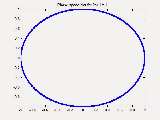
$U(x) = \dfrac{1}{2}x^2 + \dfrac{1}{3}x^3 + \dfrac{1}{4}x^4 +...+ \dfrac{1}{2n+1}x^{2n+1} $

 Note, we terminate at the index 2n+1 because otherwise the solutions diverge. The logic of such divergence is easy to understand: The force is always repulsive and further the oscillator moves, greater is the repulsive force. The MATLAB codes are attached below for the interested readers. The four resulting solutions are given below:

It is interesting to point out that the differential equations evidently become stiff under the effect of higher order nonlinear terms. The simplest way to account for it is to use the ode23s differential equation solver in MATLAB. The ode45 solver that has been used to plot these results utilize the adaptive Runge-Kutta algorithm (Runge-Kutta-Fehlberg), and can be easily implemented in a C / Fortran code. However, implementing the C / Fortran analogue of ode23s is not very trivial.

I will try to upload the results with ode23s solver for a better comparison of the effect of nonlinearity. Until then, you can use the ode45 solver codes attached below.

The MATLAB codes are given below:

main file
function file

Phi-4 model for Nose-Hoover thermostatting scheme

For the last couple of weeks I have been working on the $\phi^4$ conduction model. The model is very unique. Many works have followed Aoki & Kusnezov's work on finding thermal conductivity of this system. Prof. William Hoover has used this model to show that the Hamiltonian thermostats fail to promote heat flow.

I have written a code for those in need for $\phi^4$ model in thermal equilibrium. Thermal equilibrium is implemented using Nose-Hoover thermostat. Only a part of the system is thermostatted. The c-code is attached for those in need.

Feel free to email/comment if you find any error or have any doubts.

Link is: Nose_Hoover_Phi4_Model_C_File

Making US based NTSC Television work in India

I recently got a US make Samsung HD-LED television. In India we have PAL signal while in US they use NTSC signal. Both the signals are not compatible and as a result, your new TV may not display accurate colors. Here is how to make it work in India:

1. Do not panic in the beginning. If you receive a black and white or distorted display, do not panic. Chances are highly unlikely that you have received a faulty television. So be patient and do a lil bit of study
   
   
2. Check the voltage rating of your TV. Most TVs these days support 100-240V connection. Just to be on a safer side read the manual. In case your manual suggests a 100-110V input then get a power down transformer. Get it from a reputed company or your TV may go woof! Be sure to check the power rating of your TV. What I mean is, check the power consumption. If consumption is 50W then get a transformer of power rating 100W and NOT LESS. Getting a higher power rated step-down voltage transformer should be  your first step
   
   
3. If the display is black and white, you have two options:
   
•  Get a PAL to NTSC converter. There are plenty of these converters starting from 2,000 Rs to 30,000 Rs. It depends on how much you want to spend on these converters. I did some research on Rs 2,000 Mini NTSC - PAL converter. The link is: here. The problem is, I could not find any reviews on the product from India and the ones available on amazon.com are not good. Another downside is the quality. It cannot convert to hi-def standards. So, I decided to chunk this option.
  
• This second option is probably the easier one. I had a NORMAL (not HD) Videocon D2H service in home. So, I decided to drop a facebook message to Videocon's support page. Their response was prompt. A service engineer visited my home the very next day. We came to the conclusion that NORMAL (non HD) Videocon D2H is not compatible with NTSC Signals. However, the engineer advised me to upgrade the service to HD and voila! It works! It only set me back by Rs. 1,400
  

 There are several D2H service providers but not all support NTSC signals in India. I suggest you take a Videocon D2H service (HD) as it is the best and cheapest option for having your US TVs work in India.

Independence and Exclusivity

The concepts of independence and exclusivity of events are intertwined in probability. Often, people get confused between these two concepts. So, the objective of this post is to clarify the difference between the two. Consider two events ${A}$ and ${B}$. The conditional probability of B when A occurs can be written as:

${ P \left( A=a|B=b \right) = \dfrac{ P \left( A = a \cap B = b \right) }{P \left( B = b \right)}}$

Now, let us say when the event $A$ occurs the event $B$ does not occur. For example: let $A$ be the event that it is day now and let $B$ be the event denoting that it is night now. So, can the events $A$ and $B$ ever occur together? The simple answer is no. This means that when event $A$ occurs, the probability of occurring of event $B$ is zero. As a result, both of these events never ever occur together. This means that both these events are exclusive. In simple terms, exclusivity of  two events implies when one of the event occurs, the other event never occurs. So, in the first equation

${P \left( A = a \cap B = b \right) = 0}$

But are these exclusive events independent? Before answering this question, let us first look at what independence of events means. Again, consider two events $C$ and $D$. If these two events are independent, occurrence of one event does not affect the occurrence of the other event. For example consider $C$ and $D$ to be the outcome of a coin toss. Let $C$ denote Heads when you throw the coin once while $D$ denote heads when you throw the coin again. So, you throw the coin once and you get a heads i.e. event $C$ occurs. Does occurrence of event $D$ in any way change? It does not. This means that occurrence of $C$ has in no way altered the chances of occurrence of event $D$. Mathematically, two events are said to be independent if:

${ P \left( A=a|B=b \right) =P \left( A = a \right)}$

Now, let us look at exclusive events and independence together. When the two events are exclusive, it means that one of the events (when it occurs, see the event $A$) alters the chances of occurrence of the other event (see the event $B$, which occurs with zero probability). Therefore, both the events are not independent. Thus, in general exclusivity implies events are not independent. There is another way of look at this problem. Since, we have stated that the events do not occur together, their intersection is zero (cf. second equation). Thus, in the first equation:

${ P \left( A=a|B=b \right) = 0 \neq P \left( A=a \right) }$

Implementation of Nose-Hoover thermostat using Predictor Corrector in Molecular Dynamics

In molecular dynamics (MD) simulations temperature can be controlled via numerous methods. Out of those methods the most popular method is Nose-Hoover (NH) thermostat. The steps that are to be followed to implement NH equations in MD using Predictor Corrector algorithm is a bit challenging. So, I decided to lay an outline for the same. The steps are:

1. Prior to entering the main MD loop, evaluate forces [through a function called force( ) ]once and initialize the damping parameters (call it ${\eta}$) at 0.

2. In the main MD loop (let us say you want N simulations) call a function [let us say integrate( ) ] that evaluates the updated position and velocities

3. Within integrate( ):
    3.1. Predictor Steps: 
          3.1.a) Evaluate force( ) and let us say is stored in a vector called ${F}$

          3.1.b) Predict the updated positions through:

 ${x\left(t+h\right) = x\left(t\right) + v\left(t\right)h + \dfrac{1}{2}a\left(t\right)h^2 + \dfrac{1}{6}b\left(t\right)h^3}$

          3.1.c) Predict the updated velocities through:

 ${v\left(t+h\right) = v\left(t\right) + a\left(t\right)h + \dfrac{1}{2}b\left(t\right)h^2}$

          3.1.d) Predict the updated forces through:

 ${F\left(t+h\right) = F\left(t\right) + b\left(t\right)h}$

          3.1.e) Evaluate whether the predicted positions satisfy the periodic boundary conditions

   3.2.  Corrector Steps:
          3.1.a) Evaluate force( ) let us say the force output is stored in vector ${F_{new}\left(t+h\right)}$

          3.1.b) Update the new force to reflect the effect from bath:

${F_{new}\left(t+h\right)=F_{new}\left(t+h\right)-\eta v\left( t+h \right)}$ 

          3.1.c) Calculate the difference between the ${F_{new}}$ and ${F}$:

  ${factor = F_{new}\left(t+h\right) - F\left(t+h\right)}$

          3.1.d) Correct the updated positions through:

${x_c\left(t+h\right) = x\left(t+h\right) + p \times factor h^2}$

          3.1.e) Correct the updated velocities through:

${v_c\left(t+h\right) = v\left(t+h\right) + q \times factor h}$     

          3.1.f) Correct the updated forces through:

${F_c\left(t+h\right) = F\left(t+h\right) + r \times factor}$

          3.1.g) Correct the updated b through:

 ${b_c\left(t+h\right) = b\left(t+h\right) + \dfrac{s \times factor}{h}}$ 

          3.1.h) Check for periodic boundary conditions with the updated corrected positions

   3.3.  Update eta with the expression using NH equations of motion

4. Repeat step 3 till N simulations are complete.

NOTE: In Gear's algorithm: ${p = 1/12, q = 5/12, r = 1}$ and ${s = 1}$
PS: Please feel free to contact if you need any help or if you find any mistakes

Matlab and C codes for a single harmonic oscillator coupled with a Nose-Hoover thermostat

A single harmonic oscillator represents a very useful case for understanding the principles of non-equilibrium statistical mechanics. Today, I finished coding in Matlab and in C. The matlab files and C file can be downloaded from the following links:
Matlab Files:
nh.m
main.m
C File:
nh.c
For running matlab file download both nh.m and main.m in the same folder and then run main.m. Matlab uses ODE45 solver, which is not that great!
Standard 4th order Runge Kutta solver is used in nh.c. Output is stored in the file hh.dat. On Linux based systems run the following commands:
1. gcc nh.c -lm -g
2. ./a.out

If you find any mistake in the code, let me know. And if you like this code, drop a message :-). In case of any queries, again drop a message. I would be happy to resolve queries.

Automated snapshots every few seconds with Webcam

I have written a few simple shell scripts to take automated snapshots using webcam every 10s. The captured snapshots are transferred to desired folder. Files older than a few days are automatically deleted.
A simple application of these shell scripts can be in enhancing security and monitoring who enters the complex. Consumes negligible cpu time. Downside is - can only be used in Linux systems, works as long as your system where webcam is connected is up and running and uses up hard disk.
FILE 1: Store the following code in  master.sh Runs an automated script to take the picture and delete snapshots older than 10 days. Performs no action for 10 seconds
-----------------------------------------------------------------------------------------------
-----------------------------------------------------------------------------------------------
#!/bin/sh
while [ 1 ]; do
    echo "Hell yeah!"
    ./webcam_take_picture.sh
    ./del_older_ten_days.sh
    sleep 10
done
-----------------------------------------------------------------------------------------------
-----------------------------------------------------------------------------------------------
FILE 2: Store the following code in  webcam_take_picture.sh Runs an automated script to take the picture and stores it in desired folder
-----------------------------------------------------------------------------------------------
-----------------------------------------------------------------------------------------------
#!/bin/bash
# Path where to store taken snapshots
STORE_PATH=/home/USERNAME/Desktop
# Device locatation of webcam many webcams have default device in /dev/video0
WEBCAM_DEV=/dev/video0
# Stored grabbed picture filename prefix
FILE_NAME_PREF=security
# gets the current date and time and adds to set filename prefix
date_cur=${\$}$(date +%k_%d_%m_%Y|sed -e 's/^ *//');
time_cur=${\$}$(date +"%T")
streamer -f jpeg -o ${\$}$STORE_PATH/${\$}$FILE_NAME_PREF.${\$}$date_cur.${\$}$time_cur.jpeg
-----------------------------------------------------------------------------------------------
-----------------------------------------------------------------------------------------------
FILE 3: Store the following code in  del_older_ten_days.sh Runs an automated script to delete snapshots older than 10 days 
-----------------------------------------------------------------------------------------------
-----------------------------------------------------------------------------------------------
#!/bin/sh
#path of the folder where files are located. To be obtained through pwd command
cd /home/USERNAME/Desktop/
#delete log files older than 10 days
find . -iname '*.jpeg' -mtime +10 -exec rm -f {} \;
-----------------------------------------------------------------------------------------------
-----------------------------------------------------------------------------------------------
Store all the files in a particular folder. To run the code: navigate to the folder where the files are stored. Open the terminal and then run: ./master.sh
If you find any bug with the code, please feel free to contact :)

Pressure-Volume relationship for ideal gas undergoing adiabatic compression

So now you know molecular dynamics and you want to implement your code for some real world problem. Let us see what is the first problem that you should attempt. You all know about adiabatic compression/expansion of gases. In general a reversible adiabatic process is isentropic i.e. there is no change in entropy during the transition. But, you also know that in reality no process is a reversible process. So, let us study what happens to the entropy when the adiabatic compression is no longer reversible i.e. the process occurs at a finite rate.

You may be wondering why an isothermal process not chosen in the beginning. The reason is very simple. Remember that the first law of thermodynamics is sacrosanct (The second law is not and is valid only in statistical limit). From first law of thermodynamics we know that:

${\Delta Q = \Delta U + \Delta W}$

Here ${\Delta Q}$ represents heat flowing into/out of the system, ${\Delta U}$ represents the change in internal energy of the system and ${\Delta W}$ represents the work done by the system. For an isothermal process, ${\Delta U}$ is zero. Therefore, ${\Delta W}$ is equal to ${\Delta Q}$. But the problem is: in molecular dynamics neither calculating heat flowing into/out of the system is trivial nor is the process of keeping the system in constant temperature. For an adiabatic process, ${\Delta Q}$ is zero and thus, ${\Delta W}$ is equal to ${\Delta U}$. The change in internal energy can be calculated very easily. For example, in case of ideal gases, it is simply equal to final kinetic energy - initial kinetic energy. Consequently, it becomes extremely simple and intuitive to employ adiabatic transition process. Similar problem is done in: Phys. Teach. 41, 450 (2003); doi: 10.1119/1.1625202. We would deal with constant temperature molecular dynamics at a later stage.

Now, that we have understood why an isothermal process needs to be avoided, let us look at the theoretical aspect of the adiabatic transition process. Again for simplicity, we are looking at an ideal gas in a configuration as shown in the figure below. Both the masses have negligible height.

The process with which we are simulating gas expansion is by removal of the mass $m$.  As a result of removal of mass, gas lying in region A expands. Let the initial state of the system be denoted by $P_0,V_0,T_0$, and the final state by $P_1,V_1,T_1$. The final state is now dependent on how is the mass $m$ getting removed. 

Let us assume that the mass $m$ is removed instantly. The initial energy of the system comprises of the internal energy of the gas + potential energy of the masses. The internal energy of an equilibrated gas is given by ${U_{gas}=PV/\left(\gamma-1\right)}$. Consider the datum to be such that the potential energy of the masses is zero. Let the gas expand up to a height of $h$. From the first law of thermodynamics, the internal energy of the system remains constant i.e.

${\dfrac{P_0V_0}{\gamma-1} =  \dfrac{P_1V_1}{\gamma-1} + Mgh}$

Now, in its final position, the pressure with the gas would be such that the force would balance the weight due to mass $M$ i.e.

${P_1A=Mg}$

The final volume can also be related to height through: ${V_1=V_0 + Ah}$. Here, $A$ is the surface area. Substituting everything back to second last equation results in:

${\dfrac{P_0V_0}{\gamma-1} =  \dfrac{P_1V_1}{\gamma-1} + P_1\left(V_1-V_0\right)}$

From this equation it is now possible to plot the Pressure-Volume diagram of the gas and integrate the PV diagram to obtain the work. Interestingly, the approach of force balancing until equilibration occurs is wrong. The reason being it is theoretically impossible to define and quantify the force during the transition process. The approach via energy as shown before is simple and easy to follow. Since, entropy is a state function, determination of increase/decrease of entropy is dependent on our ability to calculate the "state" in which the system is. We can calculate the state of the system through the method highlighted before.

In the previous part we have made an implicit assumption that post compression, given sufficient time, the system would result in a new equilibrium state which is characterized by ${P_1, V_1, T_1}$. Let us now redefine the problem. We want to calculate the entropy when there is an irreversible adiabatic expansion/compression occurring using molecular dynamics . So, the problem now becomes determination of updated Pressure $P_1$ and updated temperature $T_1$ to characterize the compressed state of the system.

We assume that the piston (which expands the gas) particles interact with the gas particles through a hard-sphere type potential i.e. upon collision with piston particles, the gas molecules are instantly reflected elastically. Now, since the piston is moving at a finite rate, the reflected velocity of the gas molecules would be their pre-collision velocity - piston-velocity. This kind of a model also ensures that work is done on the system by the piston. Rate of compression can be controlled by altering the piston-speed.  If the speed is very high, this would imply instant removal of the mass $m$ as highlighted before. A low speed indicates gradual removal of the mass $m$. I will put up MATLAB code based on the previously given format in some time.

Molecular Dynamics Simulation Code in MATLAB

While I started working on Molecular Dynamics, I wanted to take a look at a sample code. But, I could not find any code especially in MATLAB. For those who need the molecular dynamics code in MATLAB, download the attached files. Codes utilize reduced units and takes into account pairwise Lennard-Jones interaction

main.m is the main file which contains all the details about other functions
initialize.m is a function  which initializes all the variables
eval_force.m is a function for calculating force
integrate.m is a function for calculating the update position and velocities
print_init.m is a function to print initial datasets
print_traj.m is used for printing the trajectories (in LAMMPS format) which can be viewed using VMD
visualize.m is used instant visualization of results

Download link is attached below:
Molecular_Dynamics_Matlab_Lennard_Jones